Polynomial Curve Fitting

This post makes a deeper dive into the subject of my previous blog post titled Bias-Variance Tradeoff in Machine Learning models. Where the previous post used the sklearn library, I will now use the underlying mathematics to implement the same model from scratch.

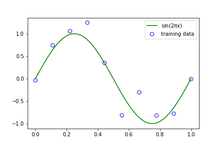
In machine learning, we assume data arises from some underlying function which is unknown and we try to estimate this function from observations (training data). In the example below, we pretend to know the underlying function \(sin(2\pi x)\) and we generate 10 data points from this function with some added noise which represents our observations. Without knowing anything about the green function in the plot, how can we fit a new function such that we can approximate the green function?

import numpy as np
import matplotlib.pyplot as plt
%matplotlib inline

def create_sample_data(fun, size, sigma):
    x = np.linspace(0, 1, size)
    t = fun(x) + np.random.normal(scale=sigma, size=x.shape)
    return x, t

def fun(x):
    return np.sin(2 * np.pi * x)

x_train, y_train = create_sample_data(fun, 10, 0.25)
x_test = np.linspace(0, 1, 100)
y_test = fun(x_test)

plt.scatter(x_train, y_train, facecolor="none", edgecolor="b",
  s=50, label="training data")
plt.plot(x_test, y_test, c="g", label="$\sin(2\pi x)$")
plt.legend()
plt.show()

We can achieve this approximation by using a polynomial model whose weights, \(\boldsymbol{w}\), need to be estimated. We can do this estimation in many ways, but the best one will resemble our underlying \(sin(2\pi x)\) function. The order of a polynomial is its highest power. So for example the expression \(x^2 + 2x + 1\) is of order 2, while \(x^3 + 2x + 1\) is of order 3. Increasing the order \(M\) of a polynomial can increase its ‘degrees of freedom’, meaning that a polynomial of order 0 is a straight line, while one with a higher order can curve in increasingly different ways as we will later see. Here, we use the function \(y(x, \boldsymbol{w})\) where,

Linear least squares regression is a method of fitting a curve which minimises the sum of squares of error between our function and training datapoints. This means that it adjusts the weights of our polynomial so that it passes as close to the blue datapoints as possible. More formally, the error is defined as:

where \(t_n\) is the \(n\)-th training datapoint. Below, we perform an experiment with varying orders of polynomial of our least square model to see the effects of increasing model complexity (in this context, a more complex model consists of a higher order polynomial).

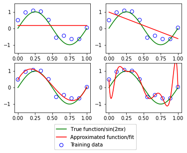
The top left plot shows a model of order=0 which results in a straight line. This model is too unsophisticated to be able to learn from our training data because changing its weights does not make it curve to fit any of the training datapoints. The next model (upper right) with order=1 is not appropriate either. The more interesting examples are the lower two plots; the lower left order=3 shows a good fit, while the lower right order=9 one shows an overfitted model.

def transform(x, degree):
  if x.ndim == 1:
      x = x[:, None]
  x_t = x.T
  features = [np.ones(len(x))]
  for degree in range(1, degree + 1):
      for items in itertools.combinations_with_replacement(x_t, degree):
          features.append(functools.reduce(lambda x, y: x * y, items))
  return np.asarray(features).T

Overfitting is when our model fits so closely to the data that it cannot generalise well when it comes to making predictions on unseen data.

class LinearRegression():
  # linear least squares regression
  def fit(self, X, t):
      self.w = np.linalg.inv(X.T @ X) @ X.T @ t
      t_hat = X @ self.w

  def predict(self, X):
      y = X @ self.w
      return y

We compute the linear least squares regression model using the Moore-Penrose pseudo-inverse of matrix \(\boldsymbol{X}\):

where \(\boldsymbol{X}\) is the \(N \times M\) design matrix with \(N>M\) and full rank (i.e. rank=m) and \(\boldsymbol{t}\) is the target matrix. Recall that an inverse of the matrix \(X\) can only be found if \(X\) is square with full rank. But since we assume that our design matrix is not square, we use the pseudo-inverse. Note that when \(X\) is square and invertible, the inverse is equal to the pseudo-inverse solution.

for i, degree in enumerate([0, 1, 3, 9]):
    plt.subplot(2, 2, i + 1)
    X_train = transform(x_train, degree)
    X_test = transform(x_test, degree)

    model = LinearRegression()
    model.fit(X_train, y_train)
    y = model.predict(X_test)
    
    plt.scatter(x_train, y_train, facecolor="none", 
    edgecolor="b", s=50, label="Training data")
    plt.plot(x_test, y_test, c="g", label="True function/$\sin(2\pi x)$")
    plt.plot(x_test, y, c="r", label="Approximated function/fit")
    plt.ylim(-1.5, 1.5)
    plt.annotate("M={}".format(degree), xy=(-0.15, 1))
    plt.legend(loc = 'lower center', bbox_to_anchor = (0.0,-0.15,1,0),
            bbox_transform = plt.gcf().transFigure)
    plt.savefig('curve_fit_2', bbox_inches='tight')

Summary

In this article, we discussed how data from the real world can be thought of to be generated from an underlying function, which we then set out to approxiate via the adjustment of weights of a polynomial function. We also explored the impact of changing the order of this polynomial function on our model and found that a delicate balance is required to arrive at a good, generalised model.

Citations:
[1] Bishop, C. M. (2007), Pattern Recognition and Machine Learning (Information Science and Statistics), Springer.
[2] PRML algorithms implemented in Python (https://github.com/ctgk/PRML).